Amateurs talk Algorithms, Professionals talk Data Cleaning

The #1 thing every assessor can do to get better results right away

Photo by Samu Lopez on Unsplash

Welcome to the third article in the Mass Appraisal for the Masses series. Prior articles:

• Part 1: The Basics

• Part 2: How Georgists Valued land in the 1900’s

In the first article we discussed the fundamentals of mass appraisal and its three goals of accuracy, consistency, and fairness, and in the second article we covered a particular method for the mass valuation of land that was employed in large American cities over a period of at least fifty years starting around the early 1900’s.

Today we’re going to pivot back to modern mass appraisal, starting with one of the single most important ways every assessor can get better results right away: by aggressively validating their sales data.

Algorithm envy

With all the fancy new technology coming out, some assessors get beaten down and feel like they aren’t keeping up with the times. Meanwhile, every IAAO conference is chock full of tech-savvy presenters (myself included) who drone on and on about shiny new methods: it’s all XGBoost this, LightGBM that, Machine learning and AI, and so on. “Algorithm envy” starts to set in, where the assessor feels that if only they had the technical wherewithal to use all these fancy new algorithms, then surely they could improve their results.

Fancy algorithms can and should be part of a balanced mass appraisal breakfast, but there’s an important lesson for technology boosters to learn (a bitter lesson if you will): data quality trumps fancy algorithms. To paraphrase a famous military slogan, “Amateurs talk algorithms, professionals talk data cleaning.”

If you have excellent data, a “good enough” method will yield excellent results; fancier algorithms are just icing on the cake. But if you have garbage data, no predictive algorithm can save you.

In the context of real estate mass appraisal, one of the worst kinds of garbage data is unreliable and misleading sales transactions, known as “invalid sales.”

Sales Validation

Sales validation is the process by which invalid sales are identified and removed from the dataset.

What’s an “invalid sale?”

An invalid sale is any transaction that is not indicative of market value. Recall our definition of “market value” from the first article in the series:

Market value of a property is an estimate of the price that it would sell for on the open market on the first day of January of the year of assessment. This is often referred to as the "arms length transaction" or "willing buyer/willing seller" concept.

The most obvious kinds of invalid sales are:

1. Sales between related parties
   E.g. in which a father ‘sells’ a house to his son at a 95% discount; this is essentially just a gift.

2. Distressed sales
   E.g. a foreclosure or other transaction forced by debt or default.

3. Government sales/purchases
   In which the government party is constrained by statute to offer or accept some arbitrary price.

However, there are other kinds of potentially invalid sales as well, such as incorrect information, multi-parcel sales, or bundled non-real estate assets (furniture, boats, jet skis) included in the transaction price.

All this is to say that an assessor should never trust a pile of non-validated sales.

Detecting Invalid Sales

How do assessors validate sales?

First, they have to get the sales. Another government office (typically the county recorder, though it can vary) will collect and share the transaction metadata—that is, the date of sale, address, location, type of property, deed, etc.—to the assessor. Usually this includes the price, but in twelve states of the union, known as “real estate non disclosure” states, the prices are not included in the records, and assessors essentially have to beg constituents to voluntarily disclose the sale prices of their homes. The only other alternative is for the assessor to buy transaction data from third party data brokers.

But even when the prices aren’t available to the assessor, the metadata itself is. Sales validation is then a process of combing through all this information and flagging anything that trips up one of the categorical rules for exclusion.

At this point we might back up and think a little about how invalid sales affect predictive models. Let’s illustrate this concretely with a simple simulated data model:

• Each house is between 1,900-2,100 square feet in size

• Houses sell for $50/sqft on average

• There’s some small natural variation in prices

NOTE: This is obviously an oversimplified toy model you’re unlikely to encounter in the real world, but just humor us as we’re just using it to make quick a point.

We generate 500 normal sales. Then we add 100 invalid sales that are half massively below (0.1x to 0.5x) and half massively above market (2x to 10x). Finally, the assessor for this neighborhood values everything using a simple $50/sqft rule. Let’s assume for the sake of argument that such valuations are basically correct. Here’s what the assessor’s model looks like before and after we add outlier sales:

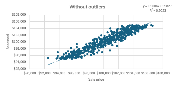
Without outliers, the assessed value has a clear and consistent relationship with the observed sale prices. This is a model that genuinely captures the behavior of the market.

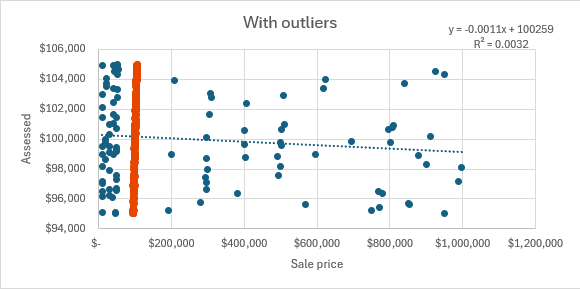
Now we throw in those 100 outlier sales:

Taken as a whole, there’s no longer any apparent relationship between assessed values and observed sale prices, because 100 of those sales are nonsensical and have no real relationship with the prevailing market value of the property.

Now, we do see a conspicuous thick line on the left hand side of the graph. If we highlight it we see that it corresponds to the “without outliers” portion of the dataset:

Now, some of you with machine learning experience might be tempted to say: “well, if we can identify the one cluster so easily, surely we can identify the other two. Perhaps we could train a model to recognize them automatically. Then, even if we’re dealing with outliers, we can at least correctly predict the prices as they lie. Isn’t this exactly what tree-based algorithms like XGBoost, LightGBM, and CatBoost excel at?”

While it’s true that those algorithms are good at picking up implicit groupings in big piles of loosely structured data, in the real world it doesn’t help much when sales data itself is corrupted in this particular way.

The key data science problem is that the physical characteristics and location of all these parcels are very similar, even for the invalid sales, but the noise from the invalid sales overwhelms the normal signal and sandblasts away the relationship between physical characteristics, location, and price. No predictive algorithm can survive that, especially in real world conditions.

Even worse, invalid sales do double damage. First, they poison your training data, so that you get worse predictions for the valid sales. Second, they poison your tests; recall from the first article that all the standard accuracy measures use sales transactions as the point of comparison. If you’re judging your valuations against invalid sales, those scores will be worse than you actually deserve. These two effects combine to tank not only your ratio study performance, but also your real-world predictive power.

Remember our giant rant against sales chasing from the first article, “sales chasing” being the practice of exactly matching the sale price for every valuation? Here’s another reason it’s a bad practice—if you just copy the latest sale price no matter what, chances are your will also copy the valuation of a few invalid sales, leading to massive over or under valuations.

Okay, so we know it’s important to identify and remove invalid sales, or else your models won’t work. How do we actually do it?

In the old days, assessors had to validate sales individually. That means looking up each property record one by one, often reviewing multiple documents from multiple government departments and/or third party data vendors, all to establish whether an individual sale was actually trustworthy and reflective of market value. Given how many sales occur in an average city each year, this was an incredibly tedious and error-prone process.

Fortunately, we can leverage statistical outliers to help make sales validation much easier.

Automated Sale Scrutiny

In a perfect world, the county recorder would provide you with pristine and perfect metadata that meticulously flags each and every invalid sale. In the real world, even after a preliminary validation pass many land mines remain buried.

While brute force predictive algorithms can’t save us from bad data, computer technology can help in cleaning that bad data up. The Center for Land Economics has built a simple script that automates part of the sales scrutiny pipeline; it’s part of OpenAVMKit, our free and open source mass appraisal software.

Here’s how it works: we group sales into clusters, ensuring that each cluster includes only sales with similar physical characteristics that all lie within a similar location. Within each of these clusters, we would generally expect market values to be roughly similar, particularly on a $/sqft basis. All we have to do to find outliers is look for anything whose $/sqft value is anomalously high or low for its local cluster.

This doesn’t do the whole job for us, but it massively cuts down on the number of sales you have to individually check. In one jurisdiction this resulted in a 96% reduction of the total search space:

Even better, we can identify certain kinds of patterns in these anomalies that not only suggest a likely cause, but also provide a recommended action for investigating further.

Vacant vs. Not Vacant

One of the most important types of sales anomalies to correct is mislabeled vacant status. This is when a parcel that was improved at time of sale is misclassified as a vacant sale, or when a parcel that was vacant at time of sale is misclassified as an improved sale.

Many mass appraisal specialists struggle with valuing land, and in my experience misclassified vacant sales are a significant contributor to that difficulty. Since vacant sales are fewer in number than improved sales, it doesn’t take many misclassifications to thoroughly poison the vacant land transaction dataset.

Fortunately, misclassified vacant status tends to stick out like a sore thumb when you look at the statistics. If a “vacant” sale is recorded as selling for a very similar price to nearby improved sales in its neighborhood, that’s a pretty good sign there could have actually been a building there at the time of sale. Furthermore, if an “improved” sale is recorded as going well below market, there’s a chance it might have been vacant at time of sale.

Recommended action:

The simplest way to check for sure is to simply look at the age of the building.

• If a property went for an anomalously low price, and the building is younger than the date of the sale, that might indicate that it was vacant at time of sale.

• If a “vacant lot” went for an anomalously high price, but there’s definitely a building sitting there now, and the building doesn’t look like recent construction, and records indicate it was constructed in 1985, probably the lot was improved at time of sale.

Vacant vs. Not Vacant is one of the single most important anomalies to get right. First, you can’t do land valuation if your “land” sales are actively leading you astray. Second, flipping the answer to the question “is there a building there?” from yes to no has a very large effect on selling price. For those reasons, these outliers tend to be particularly significant, and left unresolved, quite damaging to the predictive accuracy of models.

If aerial imagery is available in your jurisdiction, particularly on an annual basis, this becomes much easier to validate—just pull up a map, find the site for two different years, and look at it with your eyeballs—was there a building there or not? Or has the building completely changed? Aerial imagery vendors like EagleView now often include a “ChangeFinder” feature as part of their standard product suite that automatically flags and detects changes in building outlines, which is particularly useful for this kind of validation.

Other Types of Sales Anomalies

Let’s start with an overview chart. Assuming we are dealing with improved sales records, we have several variables to look at—the selling price itself, the price per square foot, and the square footage of the building. These three variables alone already give us a lot of useful hints. Let’s go through all five in turn.

1. Anomalous price/sqft, anomalous square footage

The price/sqft is very low or very high relative to the cluster, and the square footage itself is very high or low as well.

This pattern suggests that the anomaly is probably the building size itself, rather than the price. Two causes immediately come to mind:

• If the building area is under-reported, the sale price might look normal while the price/sqft appears too high

• If the building area is over-reported, the price/sqft can appear too low

Let’s look at an example:

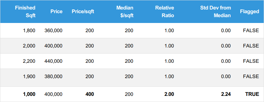
The $400,000 price range is right in line with the other sales in this cluster, but the price/sqft is double the normal amount. This is because the actual building size is only 1,000 sqft whereas the prevailing size for this cluster is ~2,000 sqft. It’s likely someone mis-recorded the building’s true size—a fact which should be easy to double check.

In the less likely event that the building truly is this small, that suggests some other unobserved factor at play that makes it go for the same price as buildings twice its size, such as much higher quality materials, a better location amenity, etc.

2. Low price, in-range square footage

In this case, the sale price itself is anomalously low, but there’s nothing remarkable about the square footage. Possibilities include:

1. Distressed/forced sale (e.g., a foreclosure, REO, or short sale) at below-market price

2. Gift/family sale well below fair market value

3. Partial-interest sale mistakenly being treated as a 100% sale

4. Severe condition issues (but mislabeled as e.g. “average condition”)

...or any other number of hidden issues that could tank a property’s sale.

Let’s look at an example:

• The normal sales in this cluster range from $360K-$420K, at a rate of $200/sqft.

• The anomaly is 2,000 sqft at $200K, yielding $100/sqft, which is half the median.

• There’s certainly something anomalous about this, and if we keep digging we’re likely to find it.

This category is one of the broadest, because so many different things could plausibly cause it. Here are some good things to look out for:

• Double-check the building characteristics, particularly age and condition.

• Pull up google street view for the building along with others in the cluster. Do the recorded characteristics seem to match what you’re seeing?

• Check transaction details for anything related to foreclosure, related-party, or partial-interest.

3. High price, in-range square footage

In this case, the sale price itself is anomalously high, but there’s nothing remarkable about the square footage.

This can have multiple different underlying causes as well, including:

1. Multi-parcel sale incorrectly classified as single-parcel

2. Non-arm’s length sale

3. Bundled intangible assets or personal property

4. Incorrectly calculated partial-interest extrapolation

In the first case, multiple parcels could have been sold together, but the record only lists the characteristics of one of those parcels, but attaches the price of the full bundle. This can sometimes be verified by looking up the transaction details of neighboring parcels, or other parcels that were sold to the same buyer, or sold around the same date.

In the third case, certain legal rights unrelated to the property itself, or movable property like furniture, vehicles, industrial equipment, etc., might have been part of the transaction.

In the last case, sometimes a parcel is purchased under fractional ownership or “partial interest.” This means that someone buys, e.g., a 20% share of the property rather than the full thing, sharing ownership with several other people. Sometimes a recorder or assessor will extrapolate a full price for the property based on the partial interest selling price—so if a 20% share of the property was sold for $100,000, then a 100% share would naively be worth $500,000, and thus the sale is evidence for a $500,000 valuation.

Partial interest transactions are tricky, however, because not all shares are created equal—one of them might come with a control premium, which gives the holder the legal right to decide what actually gets done with the land. So in the case that this 20% share came with a control premium, the actual negotiation could have been something like $20,000 for the 20% partial interest itself, and $80,000 for the control premium. That breakdown would imply that the sale counts as evidence for a total valuation of $180,000 (($20,000 x 5) + $80,000), not $500,000 ($100,000 x 5).

In any case, here’s another table showing us a concrete example of this kind of outlier:

• Normal sales in the cluster range from $360K-$420K, at ~$200/sqft

• Our anomaly is 2,000 sqft at $700K, that’s $350/sqft, 75% higher than the median

• Something extra was likely packed into this sale that we haven’t accounted for

Here are the recommended actions for this type of anomaly:

• Check the deed for extra business assets or personal property. Verify if the buyer/seller had any related party arrangement

• Check to make sure it wasn’t actually a multi-parcel sale, and that the square footage only pertains to one of the parcels

• If this was a partial-interest sale, check for a control premium, or any other factor that would artificially inflate the amount paid for this portion of the sale. If so, extrapolation from an inflated share price could be the explanation.

4. In-range price, high price/sqft, in-range square footage

In this case, the sale price and square footage are in the normal range, but the price per square foot is anomalously high.

Typical explanations include:

1. Under-reported finished area (the building is actually bigger than stated)

2. Unrecorded quality/condition upgrades (e.g. a recent renovation or addition)

In the first case, the price per square foot will be artificially inflated. Even though the square footage is in line with the cluster, the price/sqft signal might indicate that the recorded size is not correct. In the latter case, unrecorded characteristics might be enough to push the price per square foot up noticeably, even if the overall price is still within the normal range of variation.

Here’s an example:

• The normal cluster sales range from $380K-$420K at ~$200/sqft

• Our anomaly is 1,600 sqft at $400K, yielding $250/sqft, 25% higher than the median

Recommended actions:

• Double-check and verify finished area

• Double-check and verify quality and condition

• If all physical characteristics are correct, this might be perfectly valid, just a bit of natural variation.

5. In-range price, low price/sqft, in-range square footage

In this case, the sale price and square footage are in the normal range, but the price per square foot is anomalously low.

Typical causes include:

1. Over-reported finished area

2. Misclassified multi-parcel sale, but in reverse

In the first case, this means the real building area is smaller than the recorded one, so the official $/sqft value appears artificially low.

In the second case, the total recorded area includes extra square footage that isn’t truly part of the recorded sale, because it erroneously sums multiple parcels.

An example:

A Note on Clustering

There’s no reason you couldn’t reproduce everything described here, provided you have a way to cluster your sales appropriately. Our specific clustering algorithm can be found here, which I will describe briefly:

• We start with “coarse” clusters, just dividing things by user-supplied categorical variables. In other words: create one cluster for each unique neighborhood (for example), and then break those down further by each unique building type/land use.

• Additionally, we separate vacant sales and improved sales and cluster them separately.

• We divide each “coarse” cluster into narrower clusters based on user-supplied numerical variables (such as building size, land size, building quality, building condition, building age, etc.)

Rather than using off-the-shelf clustering methods such as K-means clustering, our method is specially adapted to this particular use case. It ensures that as many sales as possible are able to fit into a cluster of sufficient size, while still doing its best to minimize variation within a cluster. The trade-off is that some clusters will have more variation than others, and not all numerical features are guaranteed to be used in the clustering. We find this acceptable because most features in real estate are strongly geospatially correlated.

I note these limitations to underscore that this method provides evidence of invalidity, but not proof. That is to say, some clusters will be tighter than others, and all this method does is make it easier to quickly highlight likely problems. From there you must use your brain, rather than a computer, to confirm which sales are valid and which are not.

Going further

There’s much more that can be said on the subject of data cleaning other than sales validation, but this is one of the single largest bang-for-buck upgrades any office can make. Before reaching for advanced regression and fancy machine learning prediction algorithms, invest a little in tightening up your sales validation pipeline.