Mass Appraisal For The Masses: The Basics

How are property tax assessments calculated, and how can we know if they're fair? Let's find out!

Real estate property valuation is an obscure and mysterious topic for many, which invites confusion and even suspicion. Over the next few months I'm going to teach you more than you ever wanted to know about it.

In today's article, I begin by showing that real estate valuation need not be arcane and arbitrary, explaining its basic principles in a simple and straightforward way. I conclude by showing the reader how to perform objective tests that evaluate the accuracy, consistency, and overall fairness of any mass appraisal valuation.

The Center for Land Economics will soon publish an open source library that will allow you to perform all these statistical tests yourself as well as generate automated reports, all on real datasets pulled directly from local government open data portals.

Let us start with:

What is Mass Appraisal?

"Mass appraisal" is a fancy term for "using statistics to value a whole bunch of real estate parcels all at once." It is the counterpart to "fee appraisal," which is a fancy term for "one person spending a lot of time coming up with a value for one specific parcel at a time."

If you've ever had to "get an appraisal" for a house you wanted to buy in order to get the bank to approve the loan, that was a fee appraisal.

On the other hand, if you've ever gotten a property tax notice that sports a "valuation" for your home, that was likely the result of a mass appraisal operation. Anytime you check out the Redfin Estimate or the Zillow Zestimate, those values were also generated by mass appraisal.

Two other relevant terms of art are CAMA, standing for “Computer Assisted Mass Appraisal” (exactly what it says on the tin), and “AVM,” which stands for “Automated Valuation Model,” referring to large-scale prediction engines that cut out a lot of manual steps, often (but not always) utilizing machine learning.

Local governments and real estate listing sites are the primary practitioners of mass appraisal, but there's growing interest from state and federal regulatory bodies, researchers, as well as private interests like banks, lenders, and insurers (and ordinary citizens like you, if I get my way).

Proper mass appraisal comes down to four things:

1. Value every parcel in your jurisdiction

2. Value them accurately

3. Value them consistently

4. Value them fairly

Not only do you have to value tens or even hundreds of thousands of parcels on a deadline, you also have to prove you're getting good results, and further prove that you're not consistently under- or over- valuing certain property groups more than others.

A simple example

That all sounds quite overwhelming, so let's start by simplifying everything as much as we possibly can.

Pop quiz!

There are five houses on the same street. The five houses are physically identical in each and every way – built the same year, in the same style, all with the same quality of construction and materials, and all in the same physical condition. They're also all located along the middle of a long street in the same subdivision, and none of them have any unique amenities. All five of these properties recently sold to five different buyers, and all five of those sales were verified to be trustworthy, valid, open market transactions. By sheer coincidence, all five of those sales fell on the exact same date, January 1st of the current year.

Despite all those similarities, we observe five different selling prices:

Here's your quiz question:

What is the proper mass appraisal valuation for each house?
(Think about it for a minute, then scroll down)

.
.
.
.
.
.
.
.
.
.
.
.
.
.
.
.
.
.
.
.
.

Here's the answer:
The proper mass appraisal valuation for all five homes is $220K.

Why $220K? All five of the properties have sales attached to them, so can't we just value each one for exactly what it sold for?

That's one way to look at it, and if we had a sales tax / transfer tax on houses, that would certainly be the way to implement it. In a mass appraisal context, however, there's several problems with valuing a house at exactly what it sold for, a practice pejoratively known as sales chasing.

Sales chasing is bad

The first issue with sales chasing is that most real estate parcels don't sell in any given year, and yet we still need to come up with "market values" for them.

This becomes a little easier to grasp with an example. Let's expand our neighborhood to thirty-three homes, but keep the number of sales from the last year the same. The location, amenities, and physical characteristics of all the houses remain identical.

Now our neighborhood looks like this:

If we just copy the sale price and let that be our valuation, we are left with no method for valuing the majority of our properties, because there's no recent sale price to copy.

This is a recipe for conspicuously different side-by-side valuations, which will surely draw protests when property tax appeal season rolls around.

To illustrate this, let's say our valuations only update whenever the house is sold, regardless of how long ago that was, and then the current valuation is whatever the latest sale price was (this is actual policy in some places). Let's assume home prices go up by ~$10K per year in our neighborhood, and further that each home in our neighborhood of 33 houses has sold at least once over the last ten years. Throw in a little natural variation and that gives us a picture like this:

Now, let's highlight the upper and lower valuations (blue and yellow, respectively):

See the problem? We've got homes valued at $90K sitting right next to physically identical homes valued at $220K. Since property tax is calculated as a percent of the valuation, this means that the $220K home will be paying 2.4 times the taxes their next-door neighbor is paying, simply for the crime of buying ten years later. And this example is for a neighborhood that is a mere ten years old. When you consider that this effect exacerbates over time, and also note that homes in many American cities are fifty, sixty, or even more than a century old, you can see how bad the discrepancies can get.

Sales chasing has further problems – when enacted as an official policy it creates a strong tax incentive to never move, even if you would otherwise want to, because whatever new home you buy will see its valuation climb, while the valuation of your current home stays locked in as long as you remain.

(If you happen to be a machine learning specialist, you may have already drawn the connection between sales chasing and the ML concept of “overfitting.”)

Market Value

Okay, great, sales chasing is bad. But what are we supposed to do instead? “Follow fair market value.” Sure, but who defines what market value even is? And what makes it “fair?”

In the United States the state legislatures define it, though in practice they lean on recommendations from organizations and standards like USPAP, the Appraisal Foundation, the International Association of Assessing Officers, and their various state chapters. Here's a representative definition from the Iowa Association of Assessors:

Market value of a property is an estimate of the price that it would sell for on the open market on the first day of January of the year of assessment. This is often referred to as the "arms length transaction" or "willing buyer/willing seller" concept.

A few key terms stand out from that paragraph: “Open market,” “Arm's length transaction,” and “First day of January of the year of assessment.”

Let's start with the first two.

Of Markets and Medians

An “open market” is one where everyone has access to the same information, and an “arm's length transaction” is one where the parties don't have any special relationship or undue leverage over one another.

This means we want to filter out all the transactions between e.g. a father and son where a $5,000 “sale” is essentially a gift. Then we kick out distressed sales like foreclosures and bank auctions. In many jurisdictions you’ll also exclude multi-parcel transactions as well as sales that include a non-trivial amount of personal or moveable property. What you're left with are normal real estate transactions between parties with approximately equal bargaining power and market knowledge. Those are the transactions we’ll use to define market value.

That said, there's still natural variation in those prices, as we illustrated above. Somebody will fall in love with a house at first sight because the tree swing in the backyard reminds them of their childhood, and they'll pay a little more than average. Somebody else will drive a hard bargain and pay a little less than average, etc.

You will always see some degree of variation in sale prices even for nigh-identical properties sold at the same time in the same locations. Even so, when you gather enough sales you start to see a pattern: the central tendency. It’s the value that's right in the middle of everything.

Instead of chasing individual sale prices, mass appraisal chases the central tendency. There’s several different ways to model this, but “median sale price per square foot of living space” is by far the most popular.

Next, let's talk about "January 1st." Why does a valuation need a date?

Freezing in January

We've demonstrated above that time alone can be a significant factor in market prices. But even if we only look at sales within a given year, there will still be an irreducible bit of variation due to seasonality – prices tend to peak in spring when the market heats up, and hit a low in winter as it cools off. Here’s a graph courtesy of Redfin:

Source: Redfin.com

Mass appraisal specialists must therefore pick a date that their valuations are “for.” This is known variously as the "valuation date," "assessment date," or "lien date,” and the most popular choice by far is January 1st of the current valuation year. A separate date is chosen for the deadline to finalize values — typically this is a few months after the valuation date, but in a few cases can be as late as the following October. But even if you are still finalizing values in February or June or whatever, the valuations you’re coming up with are still the price you think the property would have sold for back in January.

There are several advantages to fixing the assessment date at the beginning of the year.

First, it makes valuations consistent and comparable – we expect similar homes in similar locations to have similar valuations when the valuation date is fixed.

Second, January 1st is in the middle of winter, so all your valuations will naturally target the low ebb of the market; it's always politically safer to err on the low side.

Third, you don't have to worry about hitting a moving target – any market changes after the valuation date will get picked up next year.

Finally, you have better evidence if your valuation date is behind you than in front of you. In contrast with the AVM's run by Redfin and Zillow, which are trying to predict the future, most local government property tax assessors are trying to predict the past. Guess which is easier to predict – the past or the future?

The bottom line is that mass appraisal valuations must all be fixed to a common date as a core element of achieving consistency and fairness, and the most popular date for this in the United States happens to be January 1st.

We'll touch on seasonality again when we assess the accuracy of mass appraisal models, but for now we'll move on to the second issue that time raises: long-term trends in the housing market.

Time rubs salt in all wounds

Housing inflation is a big deal. Did you know that a significant portion of core inflation is due entirely to housing? Here's some stats from Joey Politano of apricitas:

The chart above shows the Consumer Price Index (CPI) alongside housing’s contribution to CPI since the turn of the millennium. Housing has made up nearly 50% of the increase in CPI since 2000, no small feat when considering the price crash in 2008. In fact, housing’s contribution to CPI actually marginally increased during the period after the global financial crisis.

Besides location and size, the single most important variable in pricing any home in the United States over the last decade is the year in which it sold. According to the unsolicited offers I've been getting from real estate agents, my own home has doubled in price in the ten years since I bought it. There’s no way I would be able to afford to buy in my own neighborhood if I were on the market today!

Because year-over-year time inflation adds up, mass appraisal specialists must be careful with older sales. A common safeguard is thus to test valuations only against sales that occurred within a year of the valuation date. Older sales can still be used to train predictive models, but the modeler must first account for long-term price trends.

Market Value

Let’s put everything back together now that we understand the basic ingredients.

“Fair market value” is:

• the price the property would sell for

• in an open market, in an arm’s-length transaction

• on the valuation date

Now we know what we're aiming for. How can we tell if we're hitting the target?

Assessing the assessments

There are three things we want to know about any mass appraisal valuation, and all of them can be measured with simple tests.

1. Are the valuations accurate?

2. Are the valuations consistent?

3. Are the valuations fair?

There's a lot of ways we can define those, but in property tax assessor land it boils down to three different tests:

1. Accuracy is measured by ratio studies

2. Consistency is measured by horizontal equity studies

3. Fairness is measured by vertical equity studies

Let's start with ratio studies.

Getting Ratio’ed

Academics are used to measuring accuracy in terms of metrics like R-squared, machine learning specialists rely on stats like root mean squared error, while sites like Zillow publicly grade themselves by how many homes are within X% of their prediction.

For property assessors, the IAAO standard is the sales ratio study. This is the workhorse statistic of local government assessors throughout the United States.

A sales ratio is the ratio between valuation and sale price. Higher than 1.0 means the parcel is over-valued, and lower than 1.0 means the parcel is under-valued. The sales ratio study aggregates sales ratios across the jurisdiction.

Here's a quick example from our pop quiz:

We have five ratios here – two slightly below 1.0, two slightly above 1.0, and one that is exactly 1.0. We will use these ratios to generate two new statistics: the median ratio, and the coefficient of dispersion, or COD. These two statistics tell us how good our overall valuation is.

The median ratio measures accuracy, whereas the COD measures precision. To illustrate, here’s a nice graphic from sketchplanations:

Image: Jono Hey, Sketchplanations

In the above illustration, accuracy is how close the average position of all the points is to the center of the target. So if you have a median ratio of 1.0, you’re “centered over the target.” But this tells you nothing about how tight your grouping is, because you could all your sales ratios could be extremely close to 1.0, or they could all be very far away, but equally balanced in both directions such that the median is still 1.0. The median ratio mostly just tells you if your valuations suffer from a pervasive over- or under- valuation bias. Many assessors intentionally target a median sales ratio slightly under 1.0, such as 0.9 or 0.95, and some jurisdictions’ regulations even mandate undershooting.

Whereas the median ratio measures accuracy, the COD measures precision.

Precision is how close your predictions are to one another, regardless of how close they are to the target. Ideally you will want both accuracy and precision—a median ratio centered nicely on 1.0 (or whatever your target value is), and a low COD.

How do you calculate COD? Depends on what kind of nerd you are.

For excel nerds:

Download this spreadsheet on Google Drive!

For computer nerds:

import numpy as np

def calc_cod(values: np.ndarray) -> float:
	median_value = np.median(values)
	abs_delta_values = np.abs(values - median_value)
	avg_abs_deviation = np.sum(abs_delta_values) / len(values)
	cod = avg_abs_deviation / median_value
	cod *= 100
	return cod

For math nerds:

Let x̃ be the median and ( x₁ … x_n ) the values. The COD is then given by:

\(\text{CoD} = 100 \times \frac{\frac{1}{n}\sum_{i=1}^{n} \left| x_i - \tilde{x} \right|}{\tilde{x}} \)

If we run that calculation on our ratios from the quiz, we get this:

Median ratio: 1.00
Coefficient of dispersion: 5.6

That's a median sales ratio of 1.00, which is nicely balanced, with only 5.6% dispersion, well within acceptable limits. Keep in mind this is just a toy example – five sales is far too small a sample for a real-world ratio study, but it’s fine for illustrative purposes.

What’s a good COD? State and local regulations for ratio study tolerances vary by jurisdiction and property class, but these are the international guidelines published by the IAAO:

Source: IAAO Standard on Ratio Studies

A note on outliers

A further wrinkle in interpreting ratio studies is the practice of outlier trimming. Many local regulations will allow for the exclusion of outlier sales – typically those outside the "interquartile range", that is, sales below the 25th and above the 75th percentile, prior to performing a ratio study. The reason given by the IAAO standard on ratio studies is:

The validity of ratio study statistics used to make inferences about population parameters could be compromised by the presence of outliers that distort the statistics computed from the sample.

For this reason it's very important to pay attention to whether a particular ratio study is "trimmed" or "untrimmed" when evaluating its results. My personal recommendation is that jurisdictions should perform both; trimmed ratio studies are useful because a few spurious outliers can make an otherwise good valuation look artificially bad, but untrimmed ratio studies will give you an unflinching perspective on where your predictions are not matching sales.

A note on time

Before we move on, let's touch back again on our previous themes, particularly regarding sales chasing, seasonality effects, and year-over-year time trends.

Imagine, purely for the sake of argument, that we have a perfectly predictable market with perfect information. That's because one day God himself came down from Heaven and gave us a book in which the 100% true Fair Market Value™ of each and every property in our jurisdiction is written for every day of the year. Assuming we are still following all our local IAAO-derived assessment procedures, how low of a COD can we expect to achieve on our ratio study, armed as we are with divine cheat codes?

The surprising answer is: not zero.

Example time. Let's take the same five houses from our pop quiz, and this time we'll say that actually they sold on five different days, instead of all on January 1st. Here they each sold on the 1st day of January, April, July, October, and December 31st, respectively, in a fast-moving market where home prices steadily increase by $40K a year.

Now it's January 1st of the following year. What should each of these physically similar, similarly located homes be valued at? God's book tells us it's $240K for each and every one of them. And lest we doubt the word of the Lord, this is confirmed by empirical evidence – that's exactly what real estate agents are listing these houses for, and what buyers are offering.

Okay, great, pencils down! We have perfect information and God is literally on our side. Let's do our ratio study:

Median ratio: 1.09
Coefficient of dispersion: 5.5

Huh.

Is it really the case that, even with privileged access to the secrets of the universe, we can't get an untrimmed COD value below 5.5%? I mean, we’re not complaining—most assessors would kill for statistics that good—but are you telling me we really can't improve on this even under ideal conditions?

I'm afraid so, at least for the values in this example, because of the fundamental nature of the test itself. We are statutorily required to value as of January 1st, on which date each of these homes would really and truly sell for $240K in an open market.

Remember that for the sake of this argument these are platonically correct valuations, and they exactly match what is happening in our toy market. To drive the point home, let’s take for granted that after we finalize our valuations on January 1st, the very next day on January 2nd, all five homes will instantly sell to five independent buyers for exactly $240K.

How can it possibly be that even when we have perfect evidence and perfect valuations, we still didn’t achieve a perfect score?

Because we don’t test valuations against God’s book, but against sales.

It’s still January 1st, and all we have is the sales "as they lie"—prices that reflect slightly different market conditions than those present on the valuation date. (Some local regulatory variations may allow for ratio studies against "time adjusted" sales, but most don’t, and that’s beyond the scope of this article, anyways). We minimize time distortion by only testing against the last year of sales, but even within a single year, market movement alone will affect our test scores.

The upshot of this is that you should not expect CODs to reach zero under any circumstances, even in fantastic models. The market is just fundamentally noisy, and that's okay. Savvy readers will have noticed in the above chart that the IAAO publishes minimum COD thresholds for this very reason — incredibly low COD’s are often a sign of sales chasing.

In actual practice, your own prediction error will tend to swamp the irreducible error that comes from the noise, timing of the market, and the structure of ratio studies. If you ever find yourself butting up against this kind of theoretical minimum error, you know you’ve done the best you possibly can.

The bottom line is that single digit CODs, especially in untrimmed models, are excellent results – so long as you're not cheating.

That's it for accuracy, at least for now. Let's move on to consistency.

Horizontal Harmony

We've already shown that it's trivial to cheat your accuracy score by sales chasing. In addition to all the reasons we've mentioned above for why this bad practice, it will absolutely kill you on another measure, which in mass appraisal is known as horizontal equity.

In recent years “equity” has become a politically charged term—equity being the “E” in DEI after all—but in the assessment world “equity” has a much older definition that long predates modern culture war; it just means “uniformity” or “equal treatment.”

In layman's terms, we're just talking about consistency. Real property should be valued consistently rather than haphazardly, and without personal bias or favoritism.

There are two kinds of equity — horizontal and vertical. We’ll discuss horizontal equity now, and touch on vertical equity later. What’s horizontal equity?

Here’s a definition by Daniel Muhammad, senior economist at the District of Colombia’s CFO’s office (source):

In the realm of property taxation, horizontal inequity exists when properties with similar economic circumstances that have the same market value have dissimilar property tax liabilities.

In practice this means you expect two identical side-by-side buildings to be valued the same.

Let’s bring back our sales-chasing example from before. It would achieve a perfect ratio study—a median ratio of 1.0 and a COD of 0.0—but would be a complete nightmare in terms of horizontal equity:

Assessors nationwide tell me that bad horizontal equity is one of the single biggest drivers of property tax protests. This makes sense—imagine that you get a high tax bill in the mail, and then you compare it with your neighbor’s. His is way lower, even though you have the same kind of house and you’re literally next door. What a rip off! This kind of feedback suggests that side-by-side consistency in valuations may be a stronger driver of perceived fairness among taxpayers than raw accuracy (sales ratios close to 1.00).

Okay great, horizontal equity is important. How do we measure it? With a horizontal equity study, of course.

Unfortunately, there is no single IAAO gold standard for horizontal equity studies like there are for the ratio study standard.

Various methods exist, which I can summarize as follows—repurpose ratio studies, break them down by property type and location, then compare the ratio study breakdowns and look for differences in median ratios. By this definition, horizontal equity is achieved when you get consistent median ratios—known in this context as “assessment levels”—across different kinds of properties and locations.

This works well enough, but it has a blind spot, namely areas that have less sales. You might have entire neighborhoods without a sale, but where you must still make valuations, and you’d still like to know whether they’re uniform across property types or not.

If we look at the definition of horizontal equity again,

horizontal inequity exists when properties with similar economic circumstances that have the same market value have dissimilar property tax liabilities.

the solution becomes obvious: directly measure the uniformity of the valuations themselves.

This has the advantage of letting us test our valuation consistency throughout our entire jurisdiction, not just in places we have sales for. I call this a horizontal uniformity study, or HUS, to distinguish it from other flavors of horizontal equity study.

When conducting a HUS we don't care about accuracy, we've already run a ratio study for that. All we care about is measuring the valuation uniformity. The steps are simple:

• Divide our jurisdiction into clusters of similarly located, physically similar properties

• Calculate the $/sqft value of each property's valuation

• Calculate the coefficient of dispersion among those $/sqft values

Property clusters will be defined based on characteristics such as: location, vacant lot vs. improved lot, building size, parcel size, building age, building quality, and building condition. Clusters of vacant land will use $/sqft of land, and clusters of improved properties will use $/sqft of livable area.

We run the COD statistic against the list of valuations for all the parcels in each cluster, with each cluster being its own bucket with its own COD. Note—we are not running COD against sale ratios here, but against the valuations themselves.

A perfectly uniform set of valuations across a single cluster should yield a cluster COD of zero (something we don’t expect to actually achieve in real life). Keep in mind that in the real world not every house is exactly the same, so you actually do expect a little variation in your side-by-side values. You just want that variation to be small, and accounted for by actual differences. This is also why uniformity is measured in terms of $/sqft, rather than total valuation.

Speaking of COD, we will rename the statistic. In practice I have found that "COD" is so closely wedded in practitioner's minds to the sales ratio study, that using the same name in a different test quickly leads to confusion. For those reasons I use the term "CHD", meaning "Coefficient of Horizontal Dispersion" in the context of a Horizontal Uniformity Study. It’s the exact same math, but the unique label helps to clearly communicate its purpose.

In any case, let’s say you run a horizontal uniformity study, you get several hundred clusters. For each of these you get a CHD statistic. I find it useful to report the following:

• The number of clusters

• The CHD value of the median cluster

• The CHD value of the 25th and 75th percentile cluster

• The CHD value of the minimum and maximum cluster

These values give a good overall picture of how consistent one's valuations are across their entire jurisdiction, even in areas not well represented by sales.

Let’s go ahead and illustrate this with another example.

Here we have two neighborhoods, BlueVille on the left, and YellowDale on the right. Within each are intermingled two kinds of properties: single family homes (red roofs) and duplexes (blue roofs). Every other aspect of the buildings is the same within their building type—all the duplexes are physically identical, and all the single family homes are physically identical. As for the neighborhoods, YellowDale is a fancier part of town than BlueVille and so the land value is about $100K more than in BlueVille for equally sized lots. Within each neighborhood, all locations are equally desirable. The dollar values you see are the local assessed values.

Now let’s check horizontal equity. Here’s how we do it:

• Group properties into clusters of similar location + similar characteristics

• Measure the CHD of each cluster

That gives us four clusters:

In this example the only variables we are clustering on is neighborhood and building type. We can stop clustering right there because in this simple example every other aspect of our properties is now identical within the same cluster.

In the real world where we have many more properties, and where the properties have more physical variation, we could and should continue to cluster on characteristics like size, age, building quality, etc. My rule of thumb for the real world is that good clusters should have no fewer than 15 parcels, but we ignore that constraint for our toy example.

We’ll assign a number to each of these clusters, and calculate the CHDs:

1. BlueVille single family  = 22.97
2. BlueVille duplexes       =  3.33
3. YellowDale single family =  1.88
4. YellowDale duplexes      =  2.02

We can tell just looking at these stats that every cluster has excellent horizontal uniformity except for cluster #1, BlueVille single family, which has a CHD of 22.97, far in excess of the others.

In a simple toy example we can easily scan all four cluster scores at once and don’t need a set of summary statistics. But in the real world, we might have dozens or hundreds of clusters, so we’ll want to boil our results down to a few stats that tell us how well we’re doing overall.

The best way to do this is to take the median CHD of all the clusters. In this case that would be 2.675, indicating very good overall horizontal equity. That said, half the clusters are better than that and half are worse, and we’d like to know how much worse. I therefore recommend the following summary stats:

• Median CHD

• 25th percentile CHD

• 75th percentile CHD

• Minimum CHD

• Maximum CHD

Those five stats will give you a good heads-up about where your overall equity is at. If you have a great median CHD, but a scarily high 75th percentile CHD, that tells you that you should go ahead and look at the results broken down by individual cluster, or better yet, paint the scores on a map to visualize where your uniformity problems are.

What’s a good CHD? There’s no established standard right now, though I find that a median cluster CHD of 15 or lower is a good rule of thumb target for single family homes.

I should note that horizontal uniformity studies will yield different statistics depending on how the clusters are drawn, with the most sensitive category being the way the neighborhood or other location boundaries are drawn. For this reason I recommend that horizontal uniformity studies mostly be used as an internal tool by assessors and independent researchers to ensure horizontal equity, rather than as a tool that is ready to be deployed by oversight committees. Future research on this subject is very welcome.

Accuracy vs. Uniformity: the eternal struggle

Ratio studies and uniformity tests both suffer from the same fundamental weakness: they’re easy to cheat.

Ratio studies can be fooled by sales chasing—just value every parcel at exactly what it sold for, so that all your sales ratios will be 1.00. Any accuracy or equity study that relies on comparing valuations directly to sales shares this vulnerability.

The horizontal uniformity test can be similarly fooled simply by giving every single property in your jurisdiction the exact same value. There’s zero horizontal variation if everything’s the same!

But you know what isn’t easy to fool? Both tests at once.

Remember this image?

There’s always going to be natural variation in sale prices, even for identical properties in the same locations. Therefore, the closer you get to exact sale prices, the further you are from the central tendency, raising your horizontal uniformity CHDs. But the closer you push valuations towards the central tendency, the further your valuations are from the exact sale prices, raising your ratio study CODs.

The beauty is that when you have to hit both targets at once, it forces you to come up with a mass appraisal model that actually captures the behavior of the market and generalizes in a way that is accurate, precise, and consistent, rather than just over-optimizing for a single metric.

That’s it for horizontal equity. Let’s move on to vertical equity.

Vertical Virtue

What is vertical equity? Here’s a definition from a presentation co-authored by Ron Rakow of the Lincoln Institute of Land Policy, and my friend and colleague Paul Bidanset, president of the Center for Appraisal Research and Technology (CART):

Vertical equity exists when sales ratios (assessment / sale price) are consistent between lower, middle, and upper-priced properties

The idea here is that if all the mansions in our jurisdiction have a sales ratio of 0.5 (valued at half what they’re selling for), while all the trailer homes have a sales ratio of 2.0 (valued at twice what they’re selling for), that’s unfair.

In an ideal world, getting better at valuation in general should naturally lead to vertical equity naturally fixing itself. In the real world, however, you will always have outliers, and there will always be a concern that those outliers tend to point in a regressive direction, shifting an unfair tax burden onto those least able to pay it.

Academics such as Christopher Berry from the University of Chicago assert that vertical equity issues in property assessments are pervasive throughout the United States, even creating an interactive map that lets you explore the whole country.

But as the saying goes, “measure twice, cut once.” How do we measure vertical inequity? With a vertical equity study. As with horizontal equity, there is not a single official standard. Rakow and Bidanset’s presentation features a quote from the IAAO statistical measures task force:

“We do not recommend one particular test over another but rather that a suite of tests be reported to support the existence or absence of vertical equity.”

The most popular statistical measures assessors use for measuring vertical equity are PRD (price-related differential) and PRB (price-related bias), and some even repurpose stats from other fields such as GINI measures. The Lincoln Institute and CART built a web app that lets you upload your own CSV dataset and run all these statistics yourself:

So how good are any of these metrics?

Rakow and Bidanset on PRD:

The PRD as a vertical equity measure is useful but somewhat flawed.
- Simple and easy to calculate, but
- Results can be distorted by a few high-priced properties that can lead to a false indication of regressivity

And again on PRB:

Some academic research has found that regression based vertical equity measures like the PRB may be prone to indicating a regressive distribution even if there is no bias present (Measures of vertical inequality in assessments, McMillen & Singh, 2022).

My favorite approach therefore is the “stratum ratio study,” which is mentioned in the IAAO standard on ratio studies and employed by the Texas Comptroller School District Property Value System, which is the big annual oversight test for local property tax appraisers.*

*Local flavor note: In Texas, they’re called appraisers, not assessors. But they’re not fee appraisers, they’re mass appraisers. Keeping local terminology straight is fun!

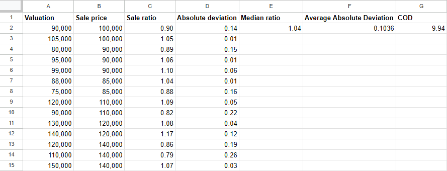
A stratum ratio study is just like any ratio study, but instead of breaking down ratio studies by geographic location or property type, you break them down by different value strata. This can be done by e.g. sale price deciles, or pre-defined buckets like “$50-100K, $100-200K, “$200-300K”, etc. You simply group your valuations and sales into these different buckets, run the ratio studies for each bucket, and look at how the median ratios and CODs differ across them. If there’s a persistent downwards slope as you move from poor to rich, you’ve got a problem.

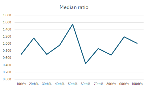
Here’s an example from Rakow and Bidanset’s presentation:

Each of the data points on the thick blue line graph is a sales ratio from a particular sale price decile.

My recommendation is to spend more time actually looking at stratum decile graphs (and visual maps of per-parcel sales ratios) than simply taking the word of a PRB or PRD statistic alone.

So now we know what vertical equity is and how to measure when it’s bad. But what actually causes it?

Causes of Bad Vertical Equity

There’s a lot of research on the subject, and four consistent findings are:

• Artificial caps on property assessments

• Infrequent valuations

• Data limitations

• Outdated assessment methodologies

Rakow and Bidanset again:

Outdated assessment methodologies hurt vertical equity simply by generating less accurate valuations than could otherwise be achieved.

Artificial caps have a tendency to benefit wealthy properties the most, because they prevent assessments from catching up to the (very large) market values indicated by expensive sale prices.

Data limitations straightforwardly hobble models because predictive models are only as good as the data they’re built from.

Inrequent valuations, which we first discussed in the horizontal equity section, also cause vertical equity issues. When the market moves quickly, it’s often the most desirable homes that go up the most in value. When those values aren’t priced in to assessments, the tax burden shifts to poor and middle class property owners.

Let’s look at few hypothetical vertical equity study results and see what they imply.

Platonically perfect:

This is what a stratum vertical equity test looks like when every single price tier has a perfect median ratio of 1.00. This is difficult to pull off in real life and should raise suspicions of sales chasing:

Believably beautiful:

This is what a more credible excellent real-world result might look like. Not every stratum gets a perfect 1.00, but they’re all quite close, and there’s no discernible bias towards cheaper or expensive properties.

Just plain bad:

Vertical equity is the least of this jurisdiction’s problems. Their sales ratios are all over the place, suggesting they have more fundamental accuracy and consistency issues to deal with first.

Strong bias:

There are significant assessment issues here, cheaper properties are significantly overvalued, more expensive properties are significantly overvalued, and this trend is strong and persistent.

Subtle bias:

This jurisdiction has a slow but steady downwards slope to their assessments. Overall the results are pretty good, but at the tails there is a significant over/under assessment bias tilted in the favor of more expensive properties.

Tippy tails:

Everything is nice and flat for the 10th-90th percentile tiers, but—oops!—the lowest tier flips up and the highest tier flips down. That’s enough to cause vertical equity problems even if the vast majority of the assessments are perfectly fine.

In cases of strong vertical equity problems, just looking at one of these charts (or painting sales ratios on a map) can quickly make clear what the problem is.

On the other hand, we know there can also be false positives:

How can we know if vertical equity issues are real or not? Let’s run through the main scenarios, starting with real problems.

Genuine problem scenario

There are plenty of cases of genuine vertical inequity, but those deficiencies are not necessarily caused by incompetence or malice. Some causes are mundane:

1. Regression to the mean

This is a well-documented phenomenon in statistical systems where there is a bias not towards the top or the bottom but towards the middle. This affects cheap and expensive properties in opposing directions, because average properties are more expensive than the cheapest properties and cheaper than the most expensive properties. Regression to the mean tends to pull predictions for cheap properties up, and to push predictions for expensive properties down.

How to fix it:

• Catch it with vertical equity tests and fix your models.

2. Data scarcity

Models are only as good as the data, and the most plentiful data is for average properties. Assessors naturally have fewer examples at the very bottom and the very top of the market to work from, and this further drives the regression to the mean effect.

This can be exacerbated by policy choices such as real estate non disclosure laws, active in twelve states, which limit the access assessors have to property transaction data. In these states assessors must acquire sales info however they can, usually by buying it from private data brokers or simply asking property owners to volunteer information. The easiest kind of sales data to get this way is for average-priced properties, and the hardest data to come by is for expensive ones. When this leads to vertical inequity, the working and middle class pay the price in the form of higher property tax burdens.

How to fix it:

• Improve data access for assessors. It’s bizarre to mandate that assessors “assess at market value” while actively denying them access to market prices.

• Supplement data with time-adjusted older sales. In many markets, when you adjust for year-over-year housing inflation, sales from a few years ago will perform similarly to current sales and can greatly expand the evidence base you need to train your models. You should still only test against very recent sales, but modern techniques can use the last 3-5 years of sales to improve sparse datasets. We will discuss methods for how to do this in a future article.

3. Wealthy people protest their taxes the most

If a property assessor overvalues a home in a wealthy neighborhood, they will be sure to hear of it come protest season. In this way, any valuation errors on the higher end tend to get swiftly corrected, while there’s less pressure coming from the low end.

Let me be clear: everyone has the right to protest their property taxes, and there is nothing wrong with wealthy people exercising their rights. Property tax protests are a key feature that makes the whole system work, something we will cover in a future article.

The real problem is not certain people protesting more, but rather over-reliance on protest feedback as an error correction mechanism.

How to fix it:

• State property tax oversight organizations (comptroller, department of revenue, etc.) should independently test local assessment bodies with up-to-date statistical measures, with a particular eye towards vertical regressivity. Properly implemented, state oversight incentivizes assessors not to undervalue, while valuation protests incentivize assessors not to overvalue.

• Mass appraisal for the masses. Most assessors post their results online. The numerical tests are well understood and can be reproduced by anyone with a computer and the proper training. All that’s lacking is someone to put it together in an easy-to-use package, which is where we come in. Stay tuned for more.

4. Statutory issues

Some vertical equity issues have nothing to do with the mass appraisal process, but with laws.

Assigning a fair market value is only the first step in the property tax assessment process. After that there is usually a panoply of carve-outs, exemptions, and write-downs that have accumulated over many decades. So even if a jurisdiction’s fair market values are accurate, consistent, and fair, the assessed values that emerge from the statutory pipeline once all the exemptions have been taken out may not be.

In this case the distortions come not from assessments, but laws.

How to fix it:

• Map out all of the statutes that affect property valuations, and determine which ones are actually promoting the goals of accurate, consistent, and fair valuations, and which are actively harming that endeavor.

5. Actual bad behavior

Assessors are human, so we will always find people engaged in bad behavior, whether it is explicit malice, personal prejudice, or someone who just isn’t doing their job.

How to fix it:

• Sunlight is the best disinfectant. This means more transparency and open data, solid state oversight, and open source tools that allow anyone to validate their jurisdictions’ results.

• Separation of powers. The power to value property should be separate from the power to tax property. Texas’ Central Appraisal District (CAD) system is a good example—contrary to what many Texas residents believe, it is not the county who values local property, but the appraisal district. The CAD is a wholly independent local government unit, similar to an Independent School District, Community College District, or Utility District. A CAD’s only job is coming up with accurate, consistent, and fair property valuations, with zero power to levey taxes. The local governments that actually raise property taxes on the other hand, have no power to set valuations—they merely control the tax rate that is applied to the valuations handed to them by the CAD.

• Put it on a map. If someone puts their thumb on a scale to under- or over- value certain properties, that gets hard to hide when you plot all the published values on a map.

That’s it for the genuine problems with vertical inequity.

Now let’s cover the other cases, when what seems at first like bad vertical equity turns out to be an innocent numerical quirk of the test itself, and the parcels in question were correctly valued all along.

False positive scenario

There’s several causes of false positives. Here are a few I’ve encountered in my own work.

1. Misclassified vacant sales

We have a property that sold last year for $10K, but which we assessed at $100K. That’s a 10x sales ratio, which is really bad! How could this be correct?

We pull up the original records, and it looks like the property was actually a vacant lot at the time it sold, and since then the buyer has put a building on it. Other similar properties in this neighborhood recently sold for $100K, so our valuation is actually correct, but comparing the (correct) current valuation to the vacant lot’s sale price makes it look wrong.

In my own work, many individual cases of seemingly egregious vertical inequity often turn out to be caused by misclassified sales. That said, I would need to replicate this work on a larger scale before making any confident assertions about how widespread this phenomenon is or isn’t.

How to detect it:

• Dig up the original sales records if you have access to them

• If you don’t have access to the original records, check all the other recent sales for improved properties in the area. If the sale is an extreme low outlier, there’s a good chance it’s a mislabeled vacant sale

• When in doubt, pull the deed. Even in real estate non disclosure states, the deeds themselves are usually still available (albeit with the price redacted).

2. Misclassified multi-parcel sales

We have a property that sold last year for $1 million, but which we assessed at $250K. That’s a 0.25x sales ratio, which is really bad! How could this be correct?

Again, let’s look closer at that original sale. Turns out, that was actually a multi-parcel sale where the buyer purchased five contiguous parcels for $200K each, getting a nice bulk discount (similar parcels next door tend to sell individually for $250K). Unfortunately, when we ingested the data we accidentally applied the price of the whole transaction to the first parcel number in the package, dropping the other four. This incorrectly classified the transaction as a single-parcel sale for $1 million.

How to detect it:

• Dig up the original sales records if you have access to them

• If you don’t have access to the original records, check all the other recent sales. If nothing similar to this property sold for anything like the huge outlier price, there’s a decent chance it’s a mislabeled multi-parcel sale.

• Check ownership records for owner information, and see if the buyer of the parcel in question also owns adjacent parcels. Also check the dates of the ownership transfers and see if they’re all on or about the same date. This could help reveal a multi-parcel sale that wasn’t immediately apparent or correctly recorded.

• Pull the deed.

3. Timing coincidence

We’ve seen in our examples from previous sections that year-over-year housing inflation can cause sales that occurred at the beginning of the year to seem undervalued when compared to values as of the valuation date. In the case that all the sales in a poorer neighborhood just happened to occur early and all the sales in a rich neighborhood just happened to occur late, this might trigger a false positive.

How to detect it:

• Put all the sales on a map and color them by “days since sale” and see if there is any persistent geographic pattern

• Adjust for time inflation in the sales and redo the test, and see if there is still a persistent bias

The bottom line

To solve vertical equity issues we need to know:

• Is there a problem?

• How bad is the problem?

• What is causing the problem?

All three of these questions can be answered with better access to data, more rigorous tools, and the latest cutting-edge methods. We at the CLE will do our part to contribute to that effort.

That brings us to the end of vertical equity, and wraps up our discussion.

We Must be Worthy of Trust

Without the trust and support of its citizens, no property tax system can stand.

We require that valuations match the market, because we expect them to be accurate. We requires valuations to be uniform because we expect them to be consistent.
We require valuations to be unbiased because we expect them to be fair.

In this article we have established what the target is as well as how to measure whether we’re hitting it. Every tool and method we’ve outlined here is an accepted practice already in use somewhere in the country, even if some of them are not as widespread as others.

We do not pretend that these measures are perfect, nor that we cannot improve upon them. What we do assert, however, is that the tools, technology, and data that exist today are more than adequate for the task, and should only continue to improve from here.

We know what we need to do, all that remains is carrying it out.

It is in pursuit of the three principles of accuracy, consistency, and fairness that we at the Center for Land Economics will continue to educate both ourselves and the general public, slowly but surely demystifying the wild and woolly world of mass appraisal.

Thanks for reading. We’re just getting started.

Get Involved

• Are you a modeler, programmer, statistician, academic, researcher, assessor, appraiser, GIS technician, ML technician, or literally anybody else who’s interested in our upcoming open source library? Email Lars at lars@landeconomics.org.

• Are you interested in land value tax in your jurisdiction and are either associated with a nonprofit/government entity or willing to lead a movement? Fill out this form.

• Are you interested in funding our work, or do you have connections to potential funding sources? Email Greg at greg@landeconomics.org.

• Do you have a unique insight into Georgist principles and land policy that you want to share on P&P? Pitch us your story at greg@landeconomics.org.

• Do you want to help in literally any other way? Email Lars at lars@landeconomics.org.

• Leave a comment on this blog and share this post with all your friends!

And last but not least, subscribe to this newsletter if you haven’t already: